Fold Growth In More Exotic Materials
The previous section showed the increase in complexity that can arise in coupling elasticity with viscosity in a simple Maxwell material. Although there has only been a limited amount of work done on more complicated materials, the characteristics of materials with coupled elastic and viscous constitutive behaviour seem to be fundamental in allowing single layers to deform into fold systems that are irregular or even chaotic with respect to the spatial distribution of wavelengths. For some such materials localisation of buckles develop; these can combine to produce irregular fold systems. In other materials the folding processes is deterministically chaotic so that the final buckled configuration is inherently sensitive to initial conditions.
In this context we emphasize that the results of the previous section, demonstrating the development of two dominant wavelengths in a buckling Maxwell layer, are based on a linear stability analysis. If one were prone to speculation, one could perhaps contemplate that a full non-linear analysis would demonstrate that such a result is part of a period doubling sequence on the route to chaos (see for instance Holmes, 1990) even for a simple Maxwell material. We await such a non-linear stability analysis with considerable interest.
We explore some non-linear behaviour briefly below.
In searching for the origin of irregular behaviour during buckling, the role of geometric and/or physical non-linearities on the folding process has been investigated many times. Yield points or high power law exponents cause sharper fold crests; more accurate geometric modelling introduces cubic non-linearities increasing the vigour of the instability. Both refinements lead to quantitative changes; they however do not introduce qualitative changes, or more or higher complexity in the model. As mentioned above, one way of introducing complexity is by considering the competition of multiple time scales; another way is to consider non-linearities related to kinematic control of the fold amplitude through prescribed axial velocities at the fold edges (see Budd et al., 1998; Budd and Peletier, 1998). It can be shown that these constraints:
- exclude periodicity of the fold amplitude distribution at all times
- increase the fold amplitude according to a power law with a power law exponent of 1/8 and not exponentially as predicted by the linear theory and expressed in (3), and
- decrease simultaneously the axial load, and the driving force of the instability with the square root of the time.
The analysis of non-linear systems with respect to buckling single layers is divided into two categories. The first category involves the analysis of non-linear constitutive laws such as Kelvin-Voigt materials (linear spring plus viscous element in parallel) and combinations of Maxwell and Kelvin-Voigt materials (Hunt et al., 1997), softening elastic layers embedded in Maxwell materials (Hunt et al., 1996a), an elastic layer in a softening Maxwell material (Hunt et al., 1996b; Whiting and Hunt, 1997) and simple non-linear mechanical systems comprised of rigid rods linked by elastic springs (Hunt and Lawther, 1999).
These analyses lead to a number of different types of solutions for the waveforms that grow. Some are illustrated in Figure 15. A feature of many such analyses is the formation of localized packets of folds (Figure 15(c), (d)) rather than an extended periodic waveform (Figure 6(c)) that is characteristic of the classical Biot-type results.
Another aspect of these non-linear approaches is the development of chaotic features of the folding process. By "chaotic" here we mean to imply a strong dependence of the fold geometry upon initial conditions and the formation of non-periodic solutions. As an example we reproduce some of the results from Hunt et al. (1996a).
The model comprises an elastic layer supported by a special Maxwell material which provides elastoviscous resistance against vertical, but not horizontal, movement (Figure 16). Notice here that the vertical deflection of the layer is w (x) where x is the spatial dimension measured along the layer. The elastic moduli of the Maxwell material are allowed to soften as the deformation proceeds. This non-linearity allows localisations, or packages of folds, to develop in the layer as shown in Figure 15. The chaotic and fractal nature of this kind of folding process is illustrated by Figure 17. We ask: What happens to an initial condition of deformation for the layer specified by a point in the four-dimensional space (w,![]() ) where a prime denotes differentiation with respect to x? Does such an initial deformation lead to a localisation or not? And how far along the layer, measured by x in Figure 16, does the localisation occur? On a plane normal to x and distant xdiv from the origin we then plot a white dot if no localisation occurs at xdiv or a black dot if localisation does occur (see Figure 17).
) where a prime denotes differentiation with respect to x? Does such an initial deformation lead to a localisation or not? And how far along the layer, measured by x in Figure 16, does the localisation occur? On a plane normal to x and distant xdiv from the origin we then plot a white dot if no localisation occurs at xdiv or a black dot if localisation does occur (see Figure 17).
We see that as we move progressively along the layer the plot of localisation versus no-localisation adopts a fractal character. Figure 15 is in fact a plot of the various localisations that occur within the small circled area on Figure 17 for xdiv = 180. Each one of these localisations corresponds to one of the black dots within the circle and each is separated from the next by a white region in this figure. In fact, the regions shown by xdiv = 100 and xdiv = 180 are completely fractal and may be magnified indefinitely to still give a black and white banded structure (see Hunt et al., 1993 for such magnification).
This example shows a characteristic that is common to most of the approaches to buckling that involve strong non-linear constitutive relations, namely that the final buckled configuration is extremely sensitive to initial conditions since initial configurations very close to each other in (w,![]() ) space can lead to either no localisation or completely different patterns of localisation. This extreme sensitivity to initial conditions is the hallmark of a chaotic system.
) space can lead to either no localisation or completely different patterns of localisation. This extreme sensitivity to initial conditions is the hallmark of a chaotic system.
The second category involving the analysis of non-linear systems within the context of buckling of single layers involves the incorporation of microstructural evolution into the constitutive behaviour and feedback relations involving the influence of flow stress upon the microstructure.
This approach promises to provide a unifying theory of geological deformation whereby microstructural and microfabric evolution can be linked to macro-scale deformation features such as fold systems.
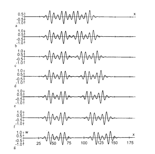
Figure 15: Localised fold packets developed in a single layer elastoviscous material with elastic shortening. ![]() is the distance measured along the layer as shown in Figure 16. w is the deflection of the layer shown in Figure 16. Each localised fold system corresponds to slightly different initial conditions.
is the distance measured along the layer as shown in Figure 16. w is the deflection of the layer shown in Figure 16. Each localised fold system corresponds to slightly different initial conditions.
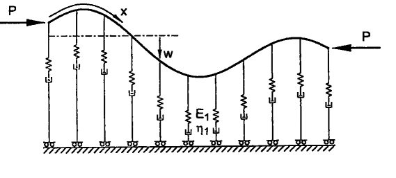
Figure 16: Geometry of the model which produces the localised fold packets of Figure 15. The elastic layer is compressed by a force P and is embedded in a viscoelastic material of Youngs Modulus E1 and viscosity
h1.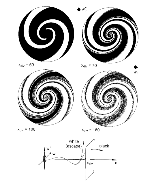
Figure 17: Plots of initial conditions (defined in this diagram by various positions in (w,w�) space) which either do (white) or do not (black) lead to the development of a localised fold package at distance ![]() along the layer. The various plots in Figure 15 are derived from the initial conditions represented in the small circle shown on the plot for
along the layer. The various plots in Figure 15 are derived from the initial conditions represented in the small circle shown on the plot for ![]() .
.
All previous work on the mechanics of folding has been at what one might call a macro-level: the buckling layer and its embedding medium are considered, in turn, to be homogeneous and isotropic with respect to their constitutive parameters and the role of microstructure is completely neglected. Yet it is clear that as rocks undergo the folding process, evolution of microstructure is intimately associated with the changing deformation history in various parts of the fold. Even more, the deformational history at each point in a deforming layer influences the patterns of crystallographic preferred orientation in concert with changes in grain shape, grain size distribution and the degree of recrystallisation. Each one of these textural and microstructural attributes is not only influenced by the deformation history but itself directly influences the flow stress. Thus, there is a feedback loop of the type.

Hence, for instance, since the deformation history at a fold hinge (consisting of pure coaxial shortening) is quite different to that on a fold limb (consisting of, initially, pure coaxial shortening followed later by non-coaxial shearing) we expect the microstructure and the crystallographic preferred orientations to be different in these two deformation regimes. Such differences have been well documented over the past seventy years (see for instance Sander, 1930). The important point here is that such microstructural and crystallographic preferred orientation differences imply different flow stress in different parts of the fold.
We explore this relationship between folding and microfabric development in a little more detail below with emphasis on grain size development during folding.
Grain size evolution relationships have been considered by authors such as Derby and Ashby (1987), Kameyama et al. (1997), and Karato et al. (1986). An interesting discussion of the phenomenology of domain boundary migration can be found on the www version of a poster by Bons et al. (1997). Recently, Braun et al. (1999) proposed an evolution relationship of the form
| (8) |
where d is the grain size, ![]() is the deformation rate,
is the deformation rate, ![]() is the characteristic strain required to reach a steady state grain size,
is the characteristic strain required to reach a steady state grain size, ![]() . This evolution law was introduced in the context of the transition (and competition) between dislocation creep and grain-size sensitive creep. The steady state grain size,
. This evolution law was introduced in the context of the transition (and competition) between dislocation creep and grain-size sensitive creep. The steady state grain size, ![]() , is given by
, is given by
| (9) |
where ![]() and
and ![]() are a reference grain size and reference stress respectively. How do grain sizes evolve in response to the highly non-linear loading history during folding? The scenarios we have in mind involve rather extreme deformations. We consider isothermal viscous flow.
are a reference grain size and reference stress respectively. How do grain sizes evolve in response to the highly non-linear loading history during folding? The scenarios we have in mind involve rather extreme deformations. We consider isothermal viscous flow.
For the viscosity we assume a power law dependence on grain size (Karato and Wu, 1993).
 . . |
(10) |
Our model folding scenario consists of five initially parallel layers of different viscosity (Figure 18). The initial geometry and the material properties are symmetric with respect to the horizontal centre line. The viscosity of the centre layer is largest and that of the outer layers is smaller. The outermost layer is present only as a computational necessity, so it is assumed to be highly compressible so that it provides virtually no impediment to folding. In all calculations we assume that ![]() and that m(1)=m(3)=0. At the beginning of the calculations (t=0), we assume that d=d0 everywhere. The layered block is strained by assuming a constant horizontal velocity, v0 = -5, at the right boundary. All other boundaries have no normal velocity and zero tangential stresses � this is equivalent to a symmetry plane. A small perturbation in the thickness of the middle layer is used to provide a trigger of the folding instability.
and that m(1)=m(3)=0. At the beginning of the calculations (t=0), we assume that d=d0 everywhere. The layered block is strained by assuming a constant horizontal velocity, v0 = -5, at the right boundary. All other boundaries have no normal velocity and zero tangential stresses � this is equivalent to a symmetry plane. A small perturbation in the thickness of the middle layer is used to provide a trigger of the folding instability.
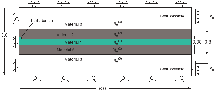
FIGURE 18. The initial state of the simulation showing boundary conditions on the solution domain.
As mentioned earlier, we are interested in large deformations which are sufficiently large that they would usually be associated with severe numerical difficulties when using updated or total Lagrangian schemes. At the heart of the problem is the ill-conditioning of the stiffness matrices due to mesh entanglement or close-to-singular Jacobians. Here we circumvent these problems by applying a finite element based material point method (Moresi et al., 2000, Mühlhaus et al., 2000)
The method uses a fixed usually regular grid and integrates the stiffness matrices and force vectors based on the information momentarily carried by a finite number of material points, ideally between 4-10 per finite element. After each time step the position of the material points (relative to a spatially fixed mesh) is updated (points may cross element boundaries) and the computational cycle continues.
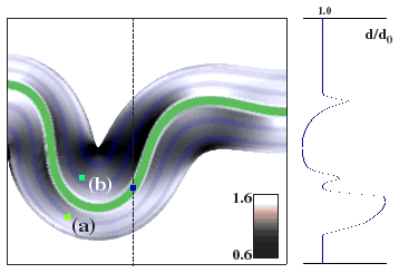
FIGURE 19. After 44% axial shortening, the material has folded and grain sizes have evolved as shown in the shading. A profile of grain size along the dashed line is shown on the right. Points (a,b) were originally located in the same vertical plane. They are fixed within the material and serve to record grain growth for a specific place during the simulation.
Figure 19 shows the deformation at 44% axial shortening of the block. The shading in the figure indicates the prevailing grain size, with dark shading indicating regions where the grains are smallest. In this example, m(2)=0, so grain size evolution does not affect the deformation. However, the deformation affects the grain growth through t in (9) and  in (8).
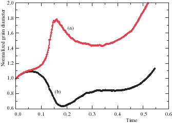
Figure 20: Normalized grain diameter for the points (a,b) shown in Figure 19 as a function of time during the simulation.
In Figure 20 we have plotted the history of the grain sizes at locations (a,b) in Figure 19. There is an initial adjustment phase in which grains everywhere grow uniformly due to the supplied compressive load. However, as the fold grows, the loading of different points such as (a) and (b) diverges. (a) is unloaded through time and shows pronounced grain growth. (b) is initially loaded and the grains become smaller but, at a later time, the stress is concentrated around the region of highest curvature away from (b).
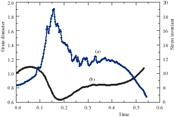
Figure 21: Deviatoric stress invariant (a), and normalized grain diameter (b) for the point (b) shown in Figure 19 as a function of time during the simulation.
In Figure 21 we plot the stress history for point (b) along with the grainsize variation. There is a clear correlation between the deviatoric stress invariants and the corresponding grain sizes indicating that, with the parameters we have chosen, the timescale of grain evolution is essentially enslaved by the structural timescale.
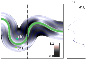
Figure 22: As Figure 19, but now the rheology is sensitive to grain size. The pattern of grain size variation is more complicated in this picture, but the magnitude of the variations is smaller than in Figure 19.
Figure 22 shows a snapshot of the deformation pattern at 44% axial shortening, but this time assuming a grain size dependence for the rheology m(2)=3. The grain size dependence of the viscosity (de)stabilizes the deformation since the viscosity is smallest where, according to (9), the stress is highest. This grain-softening effect is clearly reflected in the more localized and discontinuous appearance of the grain-size pattern in Figure 22 compared to that in Figure 19. Grain size histories for this case are very similar to those shown in Figure 20, however, the magnitude of grain size variations and stresses is moderated by the softening effects.
The plasticity like appearance of the fold deformation field is not entirely surprising. If the fold amplitudes evolve on a much larger time scale than the relaxation time of grain growth we may write ![]()
![]() ; insertion into
; insertion into
| (11) |
and rearranging gives
 |
(12) |
which is formally identical to the power law relationships of dislocation creep. In our finite element calculations we have tacitly treated grains as material objects which they are not.
The local equilibrium value of the average grain diameter is determined among other things by strain energy or the energy of stress or strain fluctuations, it is not so clear at the grain scale (eg den Brok et al., 1999). Grain boundaries seem to migrate on the microscopic scale towards local stress concentrations or equivalently towards zones of elastic strain energy concentrations. Phenomenological relationships such as (8) and (9) apply in such cases provided that the fluctuation energy is scaled by some global stress measure and that stress or strain energy gradients are not significant on the scale at which we apply our continuum description. If macroscopic stress gradients are present then we have to expect, at least in principle, a drift of the centres of the average grains of our model against the stress gradient towards zones of high stresses.
Such ideas may be incorporated into a more refined model for the dynamics of evolving grains by first introducing a grain number density n as
 |
(13) |
where ![]() is the volume fraction occupied by grains. The rate of
is the volume fraction occupied by grains. The rate of ![]() may be written as
may be written as
| (14) |
where ![]() is the relative drift velocity of the grain centres. Following the idea that grain boundaries migrate up the stress gradient we may assume for the case of microscopic isotropy
is the relative drift velocity of the grain centres. Following the idea that grain boundaries migrate up the stress gradient we may assume for the case of microscopic isotropy
| (15) |
where ![]() is a phenomenological coefficient and
is a phenomenological coefficient and ![]() is the elastic strain energy per unit volume. The influence of grain centre drift on the evolution of the spatial distribution of average grain sizes will be explored in more detail in a forthcoming paper.
is the elastic strain energy per unit volume. The influence of grain centre drift on the evolution of the spatial distribution of average grain sizes will be explored in more detail in a forthcoming paper.
At this stage it is understood however that the above energy gradient relationship is speculative and more experimental work is required to substantiate such a relationship.